With a bucketing-scheme for nearest-neighbour search in expected time O(1) this voronoi-diagram generation for 100k sites in the [0,1] unit square now runs in 30 s, i.e. it takes about 0.3 ms to insert one point.

With a bucketing-scheme for nearest-neighbour search in expected time O(1) this voronoi-diagram generation for 100k sites in the [0,1] unit square now runs in 30 s, i.e. it takes about 0.3 ms to insert one point.
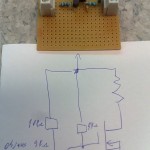
I made two small circuits today for temperature control of the extruder head on a reprap type 3D printer. The idea is to control the temperature, which needs to be somewhere between 200 and 240 C I think, using EMC2 and two parallel port pins.
The first circuit is based on the 555 and produces a square waveform with variable frequency depending on the resistance of a thermistor. At room temperature the thermistor resistance is 100 kOhms and the output frequency is below 1 Hz, and when the temperature is suitable for extrusion the thermistor resistance is about 200 Ohms which produces an output frequency of around 25-30 Hz. If the EMC2 base-thread runs with a 50 us period then it should be possible to record the frequency of this square wave using an input pin on the parallel port with an accuracy of roughly 1/500 (half a degree C?), which should suffice.
Testing the heating side of things, a wire with about 6 ohms of resistance wrapped around the extruding head, showed that a suitable DC voltage is around 8 V and produces a current of 1.3 A. The idea is to use a HAL PWM-generator to drive the base of a 337 transistor which drives the gate of an IRF610 FET that controls the current through the heating wire. By adjusting the PWM duty cycle it should be possible to control the temperature using a PID controller based on the temperature measurement.

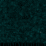
Update: now seems to work for at least 10k generators:

and a zoom-in of the same picture:

One way to compute 2D offsets for toolpath generation is via the voronoi diagram. This video shows the first (somehow) working implementation of my code, which is based on papers by Sugihara and Iri. Their 1992 paper is here: http://dx.doi.org/10.1109/5.163412, then a longer 50-page paper from 1994 here: http://dx.doi.org/10.1142/S0218195994000124, and then there's a more general description of the topology-based approach from 1999 here 10.1007/3-540-46632-0_36, and from 2000 here: http://dx.doi.org/10.1007/s004530010002
The algorithm works by incrementally constructing the diagram while adding the point-generators one by one. This initial configuration is used at the beginning:

The diagram will be correct if new generator points are placed inside the orange circle (this way we avoid edges that extend to infinity). Once about 500 randomly chosen points are added the diagram looks like this:

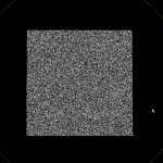
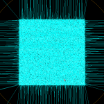
Because of floating-point errors it gets harder to construct the correct diagram when more and more points are added. My code now crashes at slightly more than 500 generators (due to an assert() that fails, not a segfault - yay!). It boils down to calculating the sign of a 4-by-4 determinant, which due to floating-point error goes wrong at some point. That's why the Sugihara-Iri algorithm is based on strictly preserving the correct topology of the diagram, and in fact they show in their papers that their algorithm doesn't crash when a random error is added to the determinant-calculations, and it even works (in some sense) when the determinant calculation is completely replaced by a random number generator. Their 1992 paper constructs the diagram for one million generators using 32-bit float
numbers, while my naive attempt using double here crashes after 535 points... some work to do still then!
CAM toolpaths tend to be based on CAD-geometry in the form of lines, circular arcs, or spline-curves and such. One way forward is to think of a curve as a lot of closely spaced points along the curve. There are also papers which describe how to extend the algorithm for line and arc generators. See the 1996 paper by Imai. There is FORTRAN code for this by Imai over here (I haven't looked at it or tried compiling it...). Held et al. describe voronoi diagram generation for points and lines in 2001: http://dx.doi.org/10.1016/S0925-7721(01)00003-7 and for points, lines, and arcs in 2009 http://dx.doi.org/10.1016/j.cad.2008.08.004. This pic from the Held&Huber 2009 paper shows point, line, and arc generators in bold-black, the associated voronoi-diagram as solid lines, and offsets as grey lines.

Held has more pictures here: http://www.cosy.sbg.ac.at/~held/projects/pocket_off/pocket.html
Note how within one voronoi-region the offset is determined by the associated generator (a line, point, or arc). It's very easy to figure out the offset within one region: points and arcs have circular offsets, while lines have line offsets. The complete offset path is a result of connecting the offset from one region with the next region.
The running log shows 1005 km this weekend!
I've run actively this year from week 13, which means 34 weeks of running/jogging so far. Or an average of 29.56km per week. Weeks 15, 19, and 37 were the low points with only 5-6 km completed (week 37 I had a fever). Week 29 (55k total) is one of the most active with a 24k long run(in central park, IIRC) in the beginning of the week, some short runs in the middle, and the Jakob half-marathon on the weekend.
At 30km/week the total should land on roughly 1200 km for this year.
There's some peer pressure on signing up for the Finlandia langlauf in February... we'll see if that happens or not.
Legs still feel a bit heavy from Sunday. This week is supposed to be a lot easier than last week, and next week is just light jogging before the D-day...
There was an uphill about 2/3rds into the last repeat which causes a jump in the HR-trace.

Long, slow, and easy.
![]()
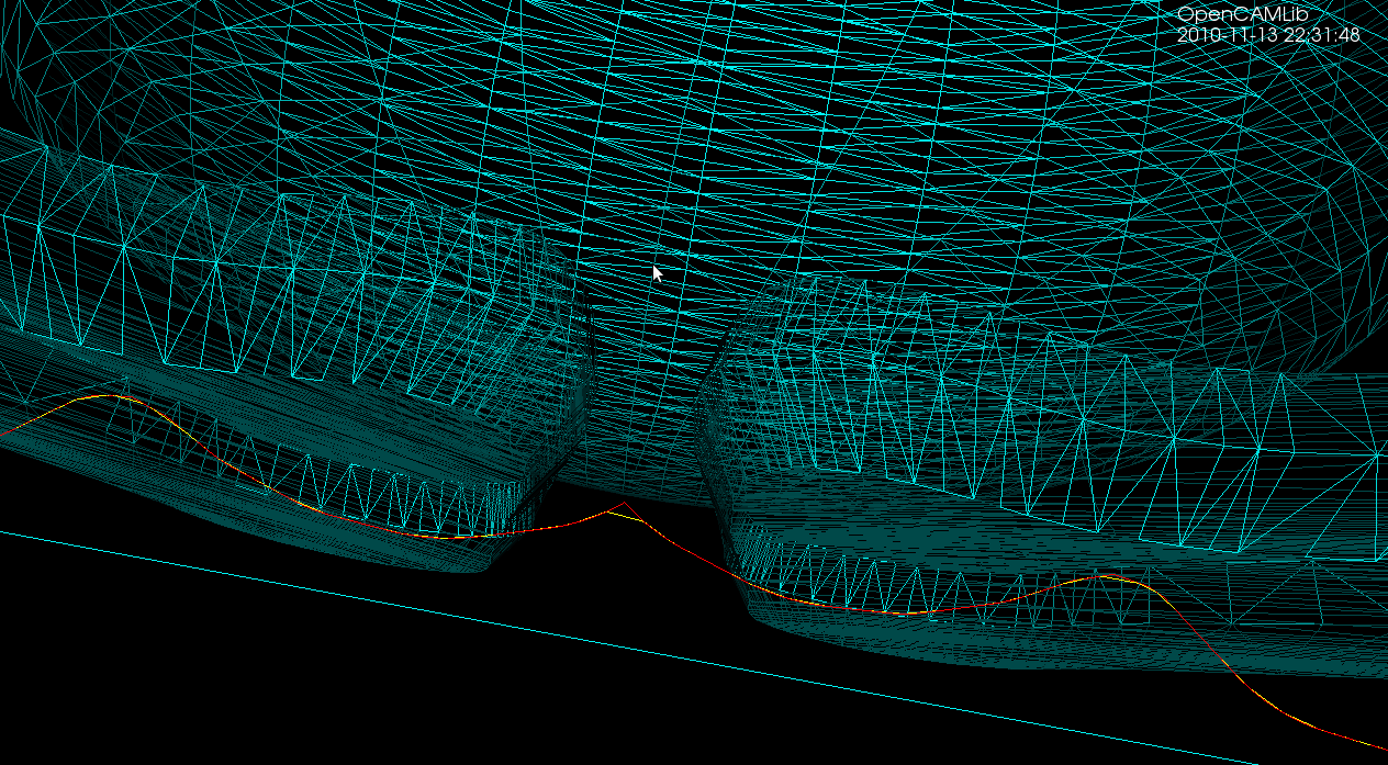
Previously the flat() predicate looked only at the number of intervals contained in a fiber when deciding where to insert new fibers in the adaptive waterline algorithm. Here I've borrowed the same flat() function used in adaptive drop-cutter which computes the angle between subsequent line-segments(yellow), and inserts a new fiber(cyan) if the angle exceeds some pre-set threshold.

This works on the larger Tux model also. However, there's no free lunch: the uniformly sampled waterline (yellow) runs in about 2 s (using OpenMP on a dual-core machine), while the adaptively sampled waterline takes around 30s to compute (no OpenMP).

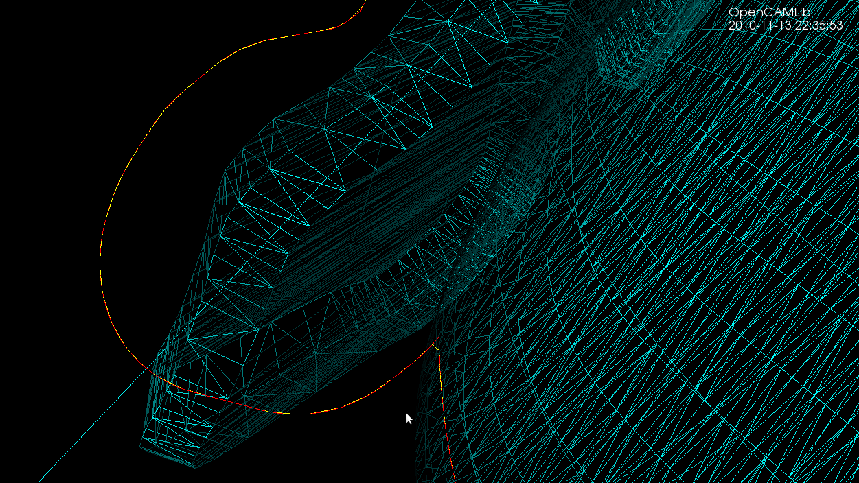
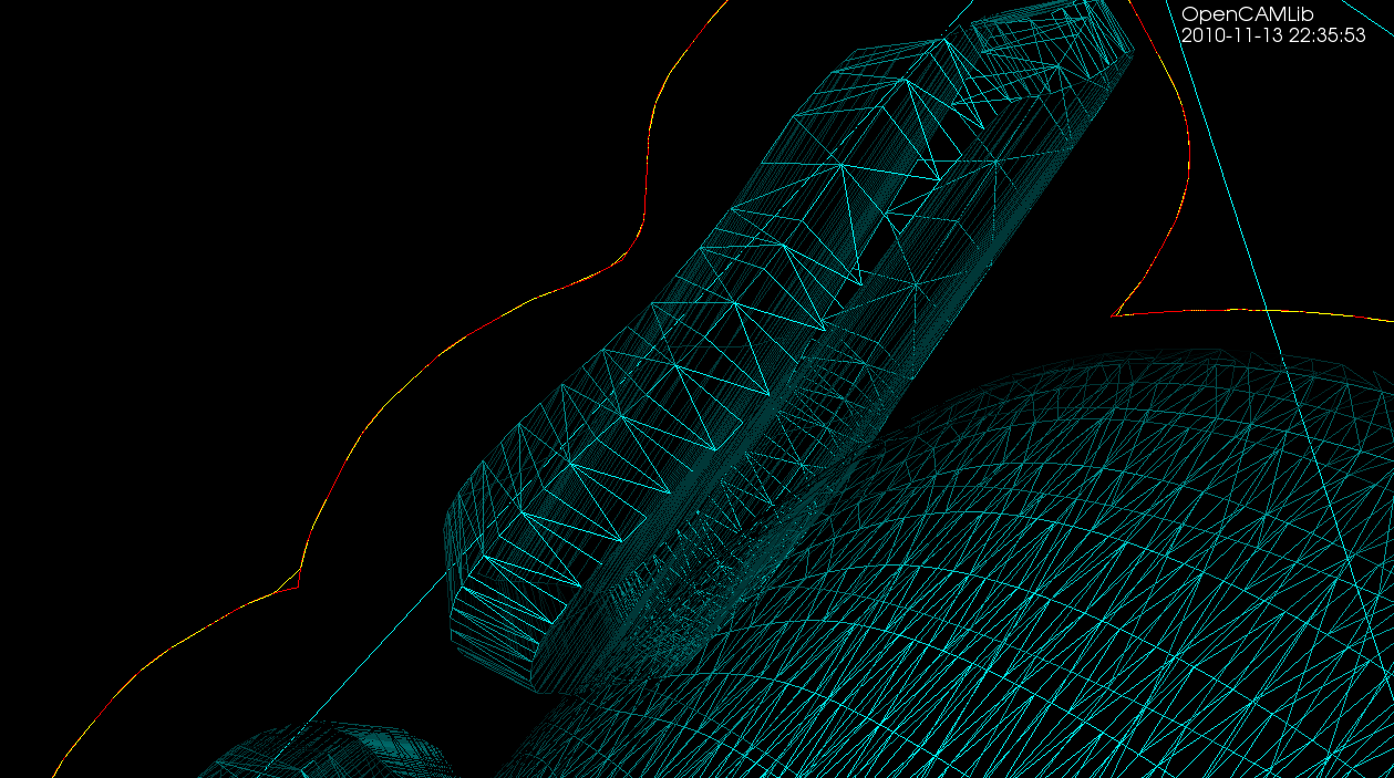
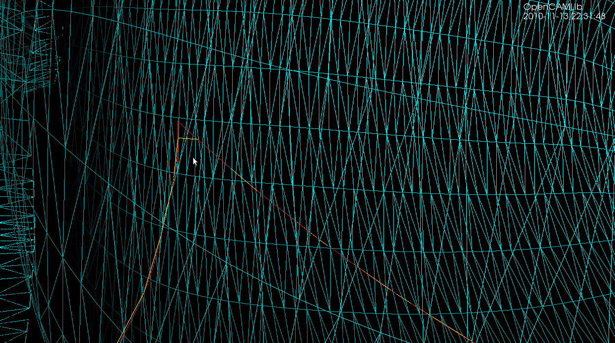
The difference between the adaptive (red) and the uniformly sampled (yellow) waterlines is really only visible when zooming in on sharp corners or other details. Compare this to adaptive drop-cutter.
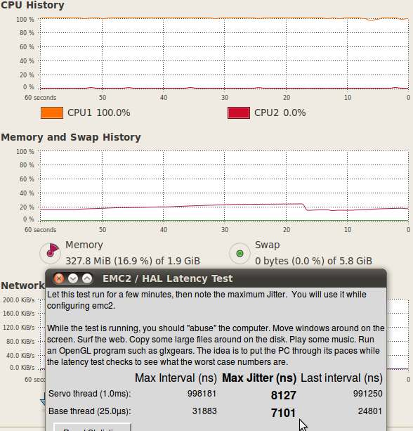
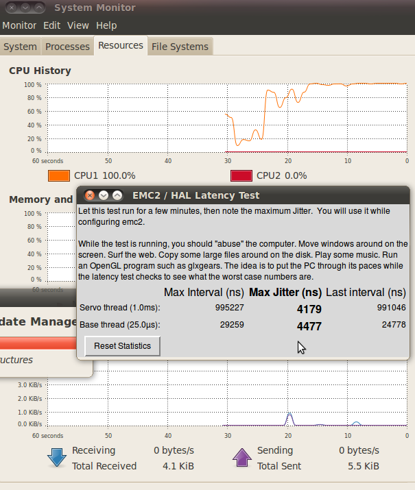
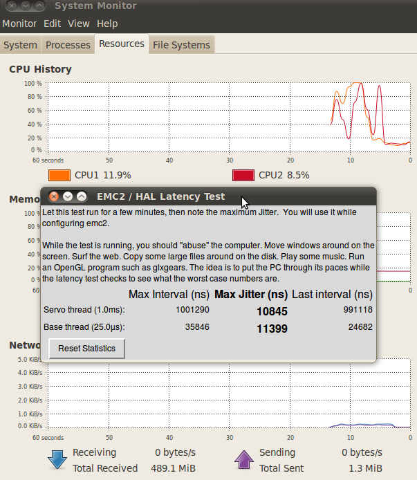
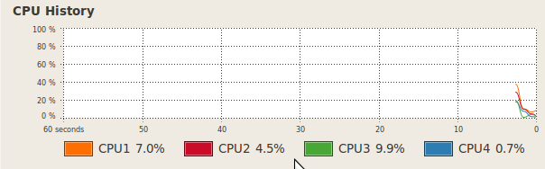
I've upgraded Ubuntu and EMC2 on the Atom 330 machine I have for controlling the lathe. The Atom 330 is a dual-core chip, but with Hyper Threading the OS can see four cores. That's not good for real-time performance, so the first thing I did was turn off HT from the BIOS. Next I did a distribution upgrade to 10.04LTS which downloaded about 1 Gig in an estimated 9 minutes (2Mb/s is OK I guess...). I then used the emc2-install script which installs the real-time kernel and emc2, and finally I edited /boot/grub/menu.lst by adding "isolcpus=1" on the kernel line. This reserves one cpu core for real-time and the other for non-real-time tasks. Without "isolcpus=1" the latency-test jitter values were easily 10k and more with a light load on the machine. With one core dedicated to real-time the jitter numbers start out at around 4k at light load and double to 7-8k under heavy load.
Here are some selected screenshots:

Next stop is getting the X and Z servos moving, as well as the hefty 2 kW spindle servo.