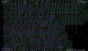
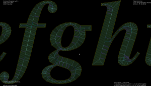
I've put together two graph filters that can be applied to the VD.
The first one detects the interior or exterior of a polygon. When the VD is constructed the polygon boundary must be input in CW order, and any islands inside the polygon in CCW order (or vice versa). This allows running other downstream algorithms only on the parts of the VD that pass the filter. Like these exterior and interior offsets:
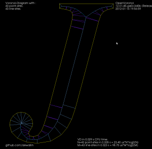
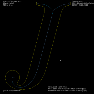
The other filter looks at the interior VD and tries to produce an approximate medial axis. We can start with the complete interior VD, such as this "J":
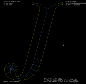
By definition the medial axis consists of "the set of all points having more than one closest point on the object's boundary". The separator edges shown in purple above can clearly be eliminated, since their adjacent/defining sites are an open line-segment and the segment's endpoint. Removing separators gives us this:
Now we can either finish here, or try to filter out some more edges to make it look better. Since we approximated smooth curves with line-segments we should try to detect which parts of the boundary are really distinct curves, and which are merely many consecutive line-segments approximating a single smooth curve. I've compared the dot-product (angle) between two consecutive segments, and applied an arbitrary threshold:
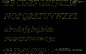
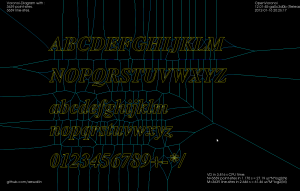
For the whole alphabet it looks like this.
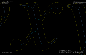
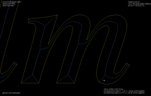
The choice of threshold value for the angle-filtering is arbitrary. In many cases such as "x" and "m" it results in small or large left-over branches. This could probably be avoided by (1) tuning the angle-threshold, (2) approximating smooth curves with a larger number of line-segments, (3) eliminating branches below a certain length, or (4) choosing a font that's made for v-carving (are there any?).
Although it's probably not right to call it a "medial axis" , the same filter applied to the exterior VD also looks interesting. It divides the plane into organic looking shapes around each letter. It could probably be used for a lot of shape analysis. For example in a smart pocketing routine to find large areas that can be cleared with a large cutter, before a smaller cutter is required for the details. Note that in addition to the geometric shape of all the blue-ish edges the diagram also holds distance-information at each point of an edge. The distance stored is a clearance-disk radius, i.e. we can draw a circle at any point of an edge with this radius, and no input geometry (in yellow) will intersect the circle.
