graph – anderswallin.net

TSP

If you have lots and lots of holes to drill on your cnc-machine you might want a TSP solver to optimize the order of the holes so as to minimize rapid movements between holes. I've written a small wrapper around metric_tsp_approx from the boost graph library and included it in opencamlib as a new class TSPSolver. Here's an example on problem "u2152" from TSPLIB95.

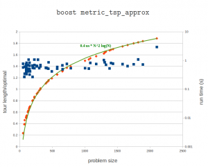
Here's a plot of the tour length compared to the known optimal tour length, as well as the run-time on my laptop (P9400 CPU). These problems range in size from 51 points to 2103 points. I might run the bigger problems on the desktop machine later. The algorithm guarantees a tour which is at worst twice the length of the optimal tour. In practice the solutions seem to scatter around 1.4 or 1.5 times the length of the optimal tour. The run times fall neatly on the predicted O(N²*log(N) curve.

A simple greedy heuristic (with better run-time?) which always selects the closest unvisited point also guarantees a tour at most twice the length of the optimal tour.

There's also a better heuristic, the Christofides algorithm, which guarantees a tour length at most 1.5 times the optimal tour length. In addition to the minimum-spanning-tree algorithm it requires a minimum cost perfect matching algorithm. I'm not sure if there is open-source code for this somewhere.

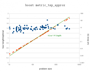
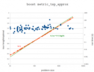
Update: here's a run on an i7-2600K cpu. The pre-factor is now halved to about 0.2 microseconds. The largest problem has 18512 cities and takes over three minutes (217 seconds) to solve.

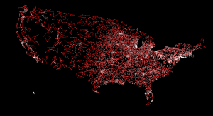
Here's 'usa13509' from TSPLIB. Cities with population at least 500 in the continental US. Presumably from 1995 or so.

Scaling (?)

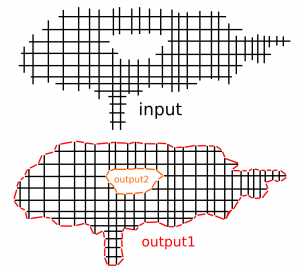
The weave point-order problem

When creating waterlines or 2D offsets using a "sampling" or "CL-point based" approach the result is a grid or weave such as that shown in black above. The black lines can in principle be unevenly spaced, and don't necessarily have to be aligned with the X/Y-axis. The desired output of the operation is shown in red/orage, i.e. a loop around/inside this weave/grid, which connects all the "loose ends" of the graph.

My first approach was to start at any CL-vertex and do a breadth_first_search from there to find the closest neighboring vertices. If there are many candidates equally close you then need to decide where to jump forward, and do the next breadth_first_search. This is not very efficient, since breadth_first_search runs a lot of times (you could stop the search at a depth or 5-6 to make it faster).

The other idea I had was some kind of 'surface tension', or edge removal/relaxation where you would start at an arbitrary point deep inside the black portion of the graph and work your way to the outside as far as possible to find the output. I haven't implemented this so I'm not sure if it will work.

What's the best/fastest way of finding the output? Comments ?!

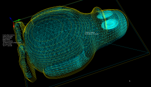
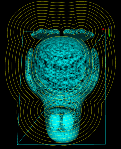
Update: I am now solving this by first creating a planar embedding of the graph and then running planar_face_traversal with a visitor that records in which order the CL-points were visited. The initial results look good:

Waterline toolpaths, part 3

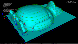
I've written a function that looks at the weave and produces a boost adjacency-list graph of it. The graph can then be split up into separate disconnected components using connected_components. To illustrate this, the second highest waterline in the picture below has six disconnected components: around the beak, belly, and toes(4). When we know we are dealing with one connected component we pick a starting point at random. I'm then using breadth_first_search from this starting point to find the distance, along the graph, from this starting CL-point to all other CL-points. We choose the point with the minimum distance (along the graph) as the next point. Sometimes many points have the same distance from the source vertex and another way of choosing between them is required (I'm now picking the one which is closest in 2D distance to the source, but this may not be correct). We then mark the newly found CL-point "done", and proceed with another breadth_first_search with this vertex as the source. That means that the graph-search runs N times if we have N CL-points, which is not very efficient...

So, compared to previously, we now have for each waterline a list-of-lists where each sub-list is a loop, or an ordered list of CL-points. The yellow lines connect adjacent CL-points.

There's still a donut-case, where one connected component of the weave produces more than one loop, which the code doesn't handle correctly.