The start was on a road wher this crazy youtuber did an everesting...
Drifted onto the wrong hill at #8, otherwise mostly ok. Not the nicest terrain to run in... +15C and sunshine.
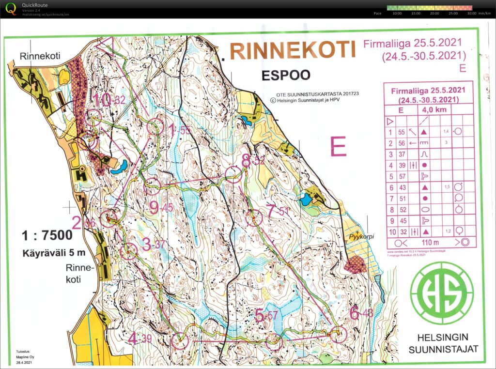
The start was on a road wher this crazy youtuber did an everesting...
Drifted onto the wrong hill at #8, otherwise mostly ok. Not the nicest terrain to run in... +15C and sunshine.

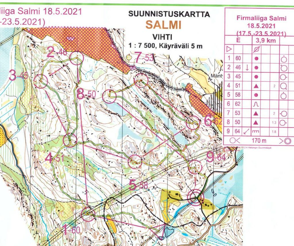
+11C and rain. Quite slippery. Maybe too safe via #4 to #2. Small loops into #6 and #8, but mostly OK orienteering.
Here's another one-inch-photodetector using OPA818 with a 2pF@5V InGaAs fiber-coupled photodiode FGA01FC. With a transimpedance gain of 4k7 Ohms the bandwidth is just over 200 MHz. A TIASim model predicts the dark-noise and response reasonably well with a parasitic capacitance (over RF) adjusted to ca 0.12 pF. The spectrum-analyzer settings weren't ideal for looking at the dark-noise which should go down to the thermal-noise of the 4k7 resistor (dashed line) - but here the instrument noise-floor prevents us from seeing that.
With new thicker solid mu-metal magnetic shields (2 layers), the clock transition in our 88Sr+ experiments shows a transform-limited linewidth of ca 10 Hz using a 72ms probe pulse. More testing to follow, as we try to lengthen the probe-pulse and search for the ultimate linewidth limit.
Farnell is now selling a dirt-cheap (28 euros or so) Multicomp fiber optic power meter, so here's a quick comparison against other power meters in the lab.
It looks like the 28 euro meter performs good enough for most tasks in the lab. The Multicomp only has a few fixed wavelength settings, while the Thorlabs is adjustable in 1nm steps.
As mentioned before, the Chi-Squared inverse cumulative distribution is used when calculating confidence intervals in allantools.
When comparing computed confidence intervals against Stable32, there seems to be some systematic offsets, which I wanted to investigate.
While allantools uses scipy.stats.chi2.ppf(), It turns out that Stable32 uses an iterative method for EDF<=100, and an approximation from Abramowitz and Stegun: Handbook of Mathematical Functions for EDF>100. This 1964 book seems to be available online from many sites. The approximation (for large EDF) for the inverse chi-squared cumulative distribution is equations 26.4.17 (p410 in the PDF) (here nu is the equivalent degrees of freedom)

Where xp is from the inverse of the Normal cumulative distribution, computed via the approximation 26.2.22 (p404 in the PDF)
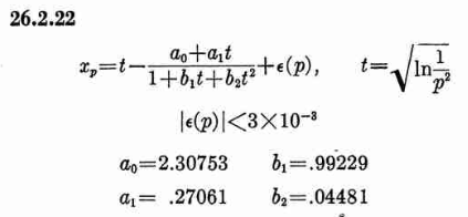
It also looks like the Stable32 source contains a misprint, where the a1 coefficient of 26.2.22 is used with two digits in the wrong order! (I did promise 'fun' in the title of this post!)
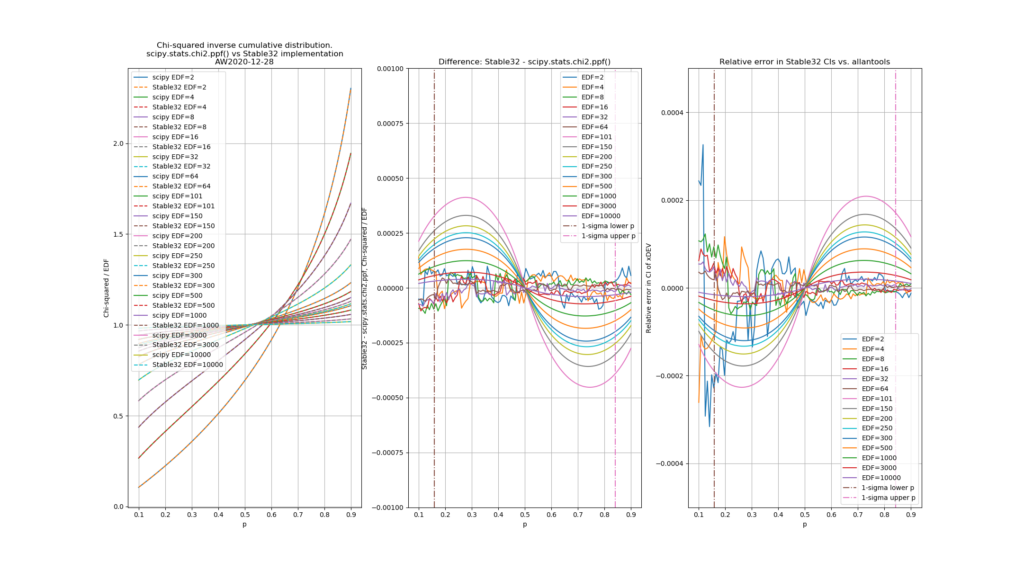
a1=0.27601 # typo in the Stable32 source code!? should be 0.27061If we plot both scipy.stats.chi2.ppf() and the Stable32 implementation for various EDF and probabilities we get the following:
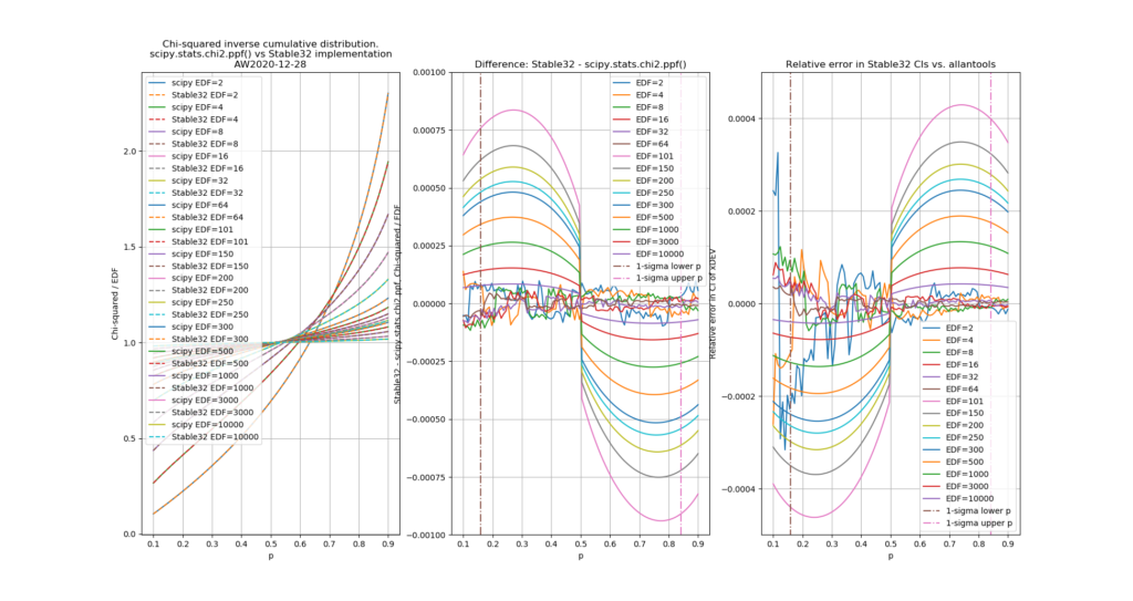
The leftmost figure shows Chi-Squared values (divided by EDF, to overlap all curves). There's not much difference between scipy and Stable32 visible at this scale. The middle figure shows the difference between the two algorithms. This shows very clearly the small (<100) EDF-region where the iterative algorithm in Stable32 produces a Chi-squared value in agreement with scipy to better than 4 digits (see the noisy traces around zero). This plot also reveals the shortcomings of the Abramovitz & Stegun approximation, together with the source-code misprint. The errors are largest, up to almost 1e-3 (in chi-squared/EDF) for EDF=101, and decrease with higher EDF. The rightmost figure shows what impact this has on computed confidence intervals - shown as relative errors. The confidence interval is proportional to sqrt(EDF/chi-squared). The dashed lines show the probabilities corresponding to 1-sigma confidence intervals, where we usually sample this function.
For 1-sigma confidence intervals we can now compare computed results with Stable32 and allantools to the comparison above of scipy and Abramovitz&Stegun + misprint.
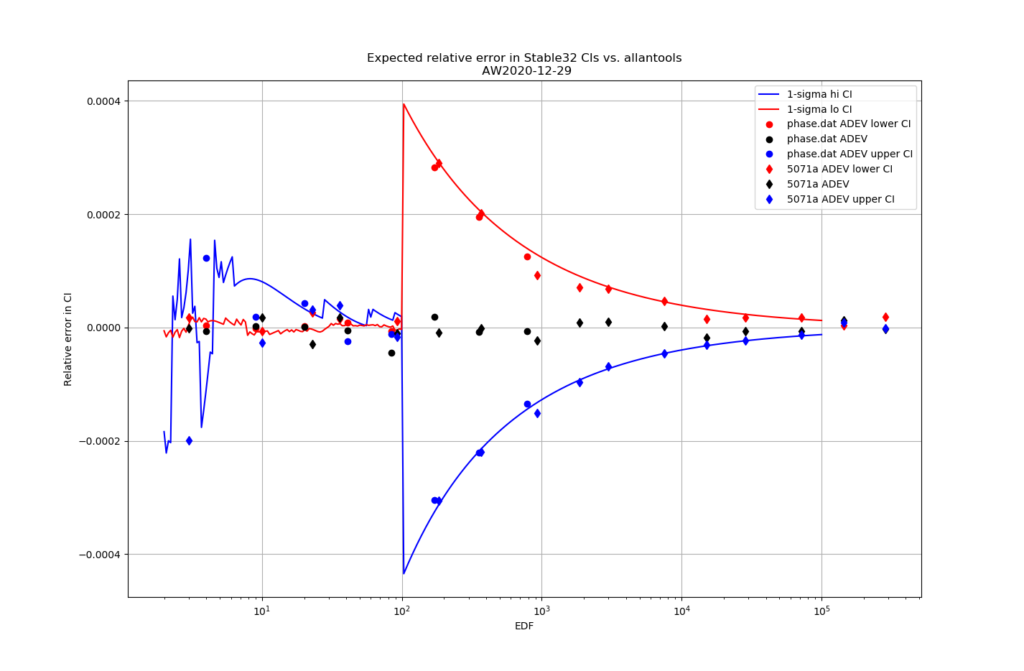
Are we having fun yet!? The comparison above between the two methods to compute the inverse chi-squared cumulative distribution seems to predict how Stable32 confidence intervals differ from allantools confidence intervals quite well! Note that Stable32 results are copy/pasted from the GUI with 5 significant digits, so some noise at the 1e-4 level is to be expected. Note that the relative error has a different sign depending on if we look at the lower or upper bound, and also depending on if we use the EDF<=100 iterative algorithm or the EDF>100 Abramovitz&Stegun+misprint approximation. For large EDF the upper bound (blue) of Stable32 is a bit too low, while the lower bound (red) is a bit too high.
Finally, the chi-squared figure and the expected confidence interval relative error figure, if we fix the misprint in the a1 coefficient:
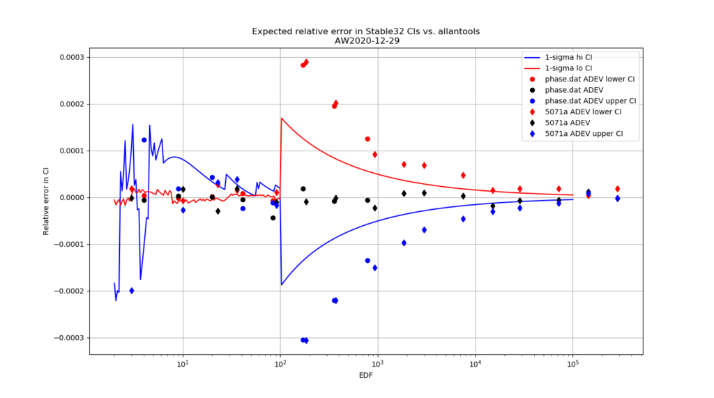
Python code for producing these figures is available: chi2_stable32.py
The approximations used by Stable32 are not (yet?) included in allantools.
Update: first production batch being tested in the lab 2020-12-17:
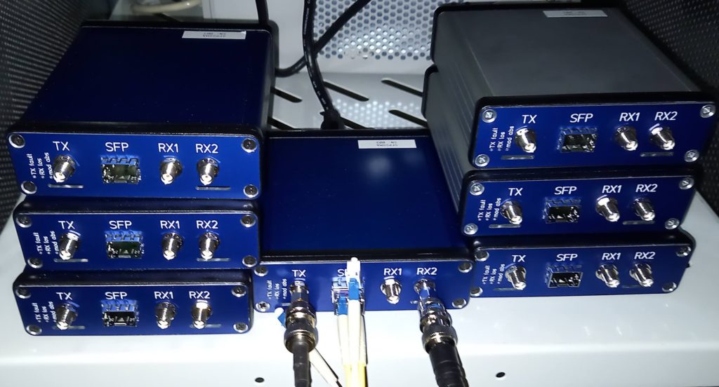
By popular demand, I've worked with Aivon to put my simple 'SFP2SMA' board (https://github.com/aewallin/SFP2SMA_2018.03) in a box, using an external Meanwell (+12V, -12V, +5V) PSU with a 5-pin DIN8 plug (model GP25A13D-R1B, Digikey 1866-1826-ND). The board can be used for simple frequency-transfer experiments together with almost any SFP-transciever. The TX SMA-connector is an input, and applies the waveform to the TX-pins of the SPF, producing modulated optical output. The dual RX SMA-connectors are driven by the SFP RX-pins, with some gain applied to produce around +10 dBm square-wave into a 50R load.
The front panel has three SFP status-LEDs: TX-fault (I've never seen this, but apparently the SFP should report if the TX-laser fails), RX LOS (loss of signal, active if you unplug the fiber), and mod_abs (module absent, active if no SFP is plugged)
After some adjustments to gains and component values the frequency-response is flat within 3 dB out to ca 400 MHz, and the ADEV looks reasonable at ca 1e-13/tau(s) (red datapoints in the plot below). These measurements were done with a CWDM SFP and a 2m single-mode loopback-fiber.
The box is a Hammond 1455L1201 (120 mm x 103 mm x 31 mm), with custom front and back panels.
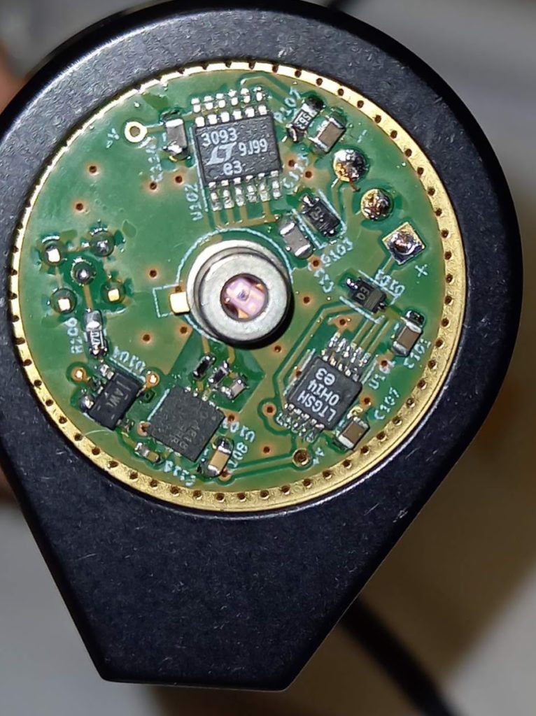
After a number of failed attempts (with HMC799, OPA859), here is a reasonably fast One Inch Photodetector using OPA818, a FDS015 photodiode, and 1.2 kOhm transimpedance. Bandwidth is above 400 MHz, with the dark-noise and frequency-response in reasonable agreement with TIASim predictions.
With the detector blocked there's quite a lot of electrical feed-through with just the spectrum-analyzer TG-output on (see blue data points, especially above 1 GHz). I tried to correct for this roughly, shown as the orange data points.